Calculate body mass index (bmi formula) in excel 2007

How to calculate ideal body weight in Excel 2007. With using microsoft excel we can calculate an ideal body weight which refers to the formula for calculating ideal body weight according to Body Mass Index. Body Mass Index (BMI) is an ideal weight calculation is based on the formula:
BMI (BMI) = Weight (kg) / (height (m) x Height (m)
If the index has been obtained from the above calculation, the next step is to match your weight criteria of BMI according to the version of the WHO (World Health Organisation):
a.BMI <18.5 means Underweight
b. BMI 18.5 - 24.9 means you ideal weight
c. BMI 25 - 29.9 means over weight
d. BMI >= 30 means obese

To calculate your ideal weight in excel do the following:
Create a table as below

How to make a sine graph in excel 2007 (plot sine wave)

Make a sine graph in excel 2007 (plotting sine wave on Excel).By using Microsoft Excel, we can easily create a graph sine, cosine graphs, charts and graphs tangent of the other trigonometric functions. Specifically discussed in this post about how to create charts in Excel sinuses that might be useful for beginner friends.

To create a graph of sin in Excel 2007, following  procedure below:
1. Create a table as below
In column A with the contents of the data point, in the following example created scale with intervals of 15 degrees.
In cell B3 enter the formula "= SIN (radians (A3))"
Copy the formula from B3 up to B27

Create cosine graph/plot cosine wave in excel

With Using Microsoft Excel, we can make a variety of curves from mathemathic functions such as trigonometric functions : sine curve, cosine, tangent, hyperbolic sine (sinh), cosec (cosecant), sec, etc.. In addition trigonometry function can also be made logarithmic curve, the exponential curve, linear curve, the curve da various other mathematical equations. Basically to make a curve of mathematical equations in excel, need data that can be sorted vertically or horizontally. By using graphics features available in Excel toolbar, then we can easily create a graph cosines

In this post will be discussed on how to graph cosine in excel 2007 (special for beginner). Please follow the procedures of cosine graph below:

How to find the matrix A if we known of Leontief matrix

How to find the matrix A if we known of Leontif matrix. This post is a continuation of my previous post about the Leontief inverse matrix, as well as to answer questions friend about the inverse matrix, which asks you about how to calculate the matrix technology if we known the Leontief inverse matrix.

If we let the technology matrix is a matrix A, and L is the Leontief inverse matrix.

L = (I - A) -1


then if L will be inverse again , Then will generate a matrix (I - A), illustrated by below equation
L-1 = (I - A) -1 = ((I - A) -1) -1 = (I - A)
then the matrix A can be calculated:
I - A = (I - A)
-A = (I - A)-I
A = absolute((I - A)-I)

Based on equation of the matrix above, then by using excel the above equation can be calculated with the following guidelines:

1. Create a table as below

How to calculate Leontief matrix in excel

Calculate the Leontief matrix in excel. Leontief matrix is a matrix that is the inverse of identity matrix minus matrix A. Leontief matrix is widely used in making the simulation or quantitative input-output analysis. In mathematical equations used to define the matrix Leontif are:

L = (I - A) -1

where:
L = matrix inverse Leontief
I = Identity Matrix
A = matrix A

By using Microsoft Excel, if we known a matrix A, then the Leontief inverse matrix can be calculated
to be more easily able to see the guidelines below:

1. Create a table matrix A and the identity matrix as below

How to calculate logarithm addition and logarithm multiplication in excel

How to calculate logarithm addition and logarithm multiplication in excel. By using Microsoft Excel, in addition  to calculate logarithm reduction and log division. Can also be done multiplication and addition of logarithms. In this post the process of logarithm addition and logarithm multiplication refers to the properties of logarithms as below:

ª log a = 1
ª log 1 = 0
ª ⁿ = n log a
ª ⁿ log b = log b n • ª
log ª ª b • c = log b + log c ª
ª log b / c = ª log b - log c ª
ª ⁿ m = m log b / log b n • ª
ª a ÷ b = log b log a
ª b log log b • c • d = c log log d ª
ª b = c log log log a b c ÷

Before applying the formula logarithms , we need using syntax of logarithm in excel as :
LOG (number, base)

With:
Number is the positive real number for which you want the logarithm.
Base is the base of the logarithm. If base is omitted, it is assumed to be 10

One of the properties of logarithms to be used is
log ª ª b • c = log b + log c ª
In order to more easily implement it, can follow the following procedure:
1. Create the table below
Columns A, B, C will contain the data, with a logarithmic base and  number
Colum D and colum W will filled with logarithm formula

How to calculate logarithm reduction and log division in excel

How to calculate logarithm reduction and log division in excel. By using Microsoft Excel, we can perform the calculation of logarithms. In this post specifically discussed about how to use a logarithmic reduction formula and the division of the logarithm.

In general, how to write formulas / functions in excel logarithms is using syntax:

LOG (number, base)

with:
Number is the positive real number for which you want the logarithm.
Base is the base of the logarithm. If base is omitted, it is assumed to be 10
.

A simple example application of the reduction formula and the distribution of the logarithm can be seen below
ª log b / c = ª log b - log c ª

To calculate in Excel can follow the following procedure:

1. Create a table as below
Column A is the logarithmic base
Columns B and C is filled with data
Column D and E will filled with logaritm formula

Calculate circumference of a circle in excel

With using excel we can find circumference of a circle. If we know the radius value, diameter value or area value then we can calculate and find circumference of a circle.

There are some formula to calculate circumference of a circle in excel, is defined on below table :

With :
A = area of cirle
r = radius of circles
d = diameter of circle
C = circumference of cirles

How to Calculate the Area of a Circle

A circle is one of the geometric shapes, sometimes we need to calculate the radius, diameter, area or circumferences of circle. With using excel we can find the radius, diameter, area or circumferences of circle  using formula below :

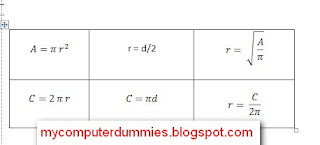
For example :

1. Create table below

There are 3 cell contain data . 

a. Cell B5 is a radius data

If we know radius value, then we can calculate the area of circle

b. Cell B9 is a diameter data

If we know diameter value, then we can calculate the area of circle

c. Cell B13 is a circumferences data

If we know circumferences value, then we can calculate the area of circle

Feature Specification and Limits of Microsoft Excel 2007

There are some new feature of Microsoft Excel 2007, but every feature has specification and limits, such as :

a. Worksheet and workbook specifications and limits
b. Calculation specifications and limits
c. Charting specifications and limits
d. PivotTable and PivotChart report specifications and limits
e. Shared workbook specifications and limit

For details every Specification and Limits , we can see on table below :

Microsoft Excel Tutorials

Microsoft Excel is a powerfull spreadsheet application that can be use for calculation of dataset, create graph, make pivot tables, and customize procedure calculation using a macro programming language called Visual Basic for Applications.

Below there are some tutorials  microsoft excel 2003 and 2007 for beginner.

Introduction

What's new in Microsoft Office Excel 2007

Microsoft Office Excel 2007 provides powerful tools and features that you can use to analyze, share, and manage your data with ease

There are some new feature in Microsoft Office Excel 2007, such as :

1. Results-oriented user interface with ribbon menu

The new results-oriented user interface makes it easy for you to work in Microsoft Office Excel. Commands and features that were often buried in complex menus and toolbars are now easier to find on task-oriented tabs that contain logical groups of commands and features. Many dialog boxes are replaced with drop-down galleries that display the available options, and descriptive tooltips or sample previews are provided to help you choose the right option.
No matter what activity you are performing in the new user interface—whether it's formatting or analyzing data—Excel presents the tools that are most useful to successfully complete that task.

2. More rows and columns, and other new limits

Calculate angles using the arcsin, Arccos, arctan in excel 2007

Arcsin function is a trigonometric function that is used to calculate the inverse sinevalue, while the arccos are inverse cosine function, and atan is the inverse tangent function.
This function is an inverse function of sin, cos, tan. In general, writing formulas in Excel can be seen below

syntax:
arc sine ---> ASIN (number)
arc cosine ---> ACOS (number)
arc tan -----> ATAN (number)

Note: a number in radians domain
To display the results of the inverse sine, cosine, tangent in degrees then the formula above needs to be simplified by multiplying by 180/PI () or by combiningthe functions DEGREES

In general the writing of ASIN(), ACOS (), and ATAN() in mathematical equations can be seen below

Example:

1. Create a table below

Convert Decimal to Octal

How to Convert from Decimal to Octal. By using Excel 2003, the decimal number can be converted into Octal (decimal to Octal). However, the function to convert decimal numbers to Octal has the some limitations of which can be seen in the syntax and description below:

Syntax
DEC2OCT(number, places)

Number is the decimal integer you want to convert. If number is negative, places is ignored and DEC2OCT returns a 10-character (30-bit) octal number in which the most significant bit is the sign bit. The remaining 29 bits are magnitude bits. Negative numbers are represented using two's-complement notation.
Places is the number of characters to use. If places is omitted, DEC2OCT uses the minimum number of characters necessary. Places is useful for padding the return value with leading 0s (zeros).
Remarks
If number < -536,870,912 or if number > 536,870,911, DEC2OCT returns the #NUM! error value.
If number is nonnumeric, DEC2OCT returns the #VALUE! error value.
If DEC2OCT requires more than places characters, it returns the #NUM! error value.
If places is not an integer, it is truncated.
If places is nonnumeric, DEC2OCT returns the #VALUE! error value.
If places is negative, DEC2OCT returns the #NUM! error value

We tried to apply the function DEC2BIN,

Create a table like below

Convert Decimal to Binary

How to Convert from Decimal to Binary. By using Excel 2003, the decimal number can be converted into binary (decimal to binary). However, the function to convert decimal numbers to binary has the some limitations of which can be seen in the syntax and description below:

Syntax :
DEC2BIN(number,places)
Number is the decimal integer you want to convert. If number is negative, places is ignored and DEC2BIN returns a 10-character (10-bit) binary number in which the most significant bit is the sign bit. The remaining 9 bits are magnitude bits. Negative numbers are represented using two's-complement notation.
Places is the number of characters to use. If places is omitted, DEC2BIN uses the minimum number of characters necessary. Places is useful for padding the return value with leading 0s (zeros).
Remarks
If number < -512 or if number > 511, DEC2BIN returns the #NUM! error value.
If number is nonnumeric, DEC2BIN returns the #VALUE! error value.
If DEC2BIN requires more than places characters, it returns the #NUM! error value.
If places is not an integer, it is truncated.
If places is nonnumeric, DEC2BIN returns the #VALUE! error value.
If places is negative, DEC2BIN returns the #NUM! error value.

Text function in excel 2003

Based on data from 2003 excel offline help, there are some text functions such as: 

ASC Changes full-width (double-byte) Bahasa letters or katakana within a character string to half-width (single-byte) characters
BAHTTEXT converts a number to text, using the ß (baht) currency format
CHAR Returns the character specified by the code number
CLEAN Removes all characters from a text nonprintable
CODE Returns a numeric code for the first character in a text string
Trust Joins CONCATENATE text items into one text item
DOLLAR converts a number to text, using the $ (dollar) currency format
EXACT checks to see if two text values are identical
FIND Finds one text value within another (case sensitive)
FIXED Formats a number as text with a fixed number of decimals
JIS Changes half-width (single-byte) Bahasa letters or katakana within a character string to a full-width (double-byte) characters


LEFT Returns the leftmost characters from a text value

Error 16 digit number in excel 2003

If you type 16 digit or more in excel 2003, example 455558977564345999 cannot be represented in Excel's numeric storage format.. If you don't need to do math with it, then prefix with a single quote to store it exactly as text.

List of error or bug in excel 2003

List of error or bug in excel 2003

1.You receive "The file may have been changed..." error message when you save a workbook to a network server in Excel 2002 or in Excel 2003

2.You cannot change a link path when an Excel Add-In is not loaded

3. Excel Abruptly Quits When You Save a Workbook

4. Unable To Read File" Error Message When You Open a Workbook and Try to Update Links

5. Using a field alias in Query does not work with some third-party databases

6. You Cannot Open Excel Files in Windows Explorer After You Use the Text Import Wizard

7. VBA Error on Macro Startup If You Open Multiple Excel Instances with RefEdit Control

8. Pivot Table Fields Do Not Function After Excel Repairs and Recovers File

9. You Receive Error Messages When You Delete Multiple Columns from a Graph

10. The CPU Usage Is 100 Percent When You Copy a Large Sheet in Excel

11. Hyperlink Syntax Does Not Save Correctly When You Save an Excel File as an HTML Page

12. Excel Stops Responding When Subtotals Are Removed

13. Edits to PivotTables Do Not Bring Back New Columns

Fix Error RAND, RANDBETWEEN, SLOPE, INTERCEPT, FORECAST, and STEYX functions in Excel 2003

Microsoft has released an update to Microsoft Office Excel 2003. This update fixes a problem in Excel 2003 that can cause the RAND(), RANDBETWEEN(), SLOPE(), INTERCEPT(), FORECAST(), and STEYX() functions to return values that are not correct. This update fixes the problem so that these functions generate the correct results.

Subtract matrix

Microsoft excel provides a function to subtract martiks. Matrix reduction process in accordance with the rules of the matrix, the matrix can be deducted if it has the same order.
Here we will try to subtract two matrix (order 4x4)

1. Create a matrix as below (only accecories brackets, can be ignored)

2. Block range to put the results of reduction (adjust the order of the matrix that will be deducted)



3. Type the formula:
= A4: C7-E4: G7



Perform array by pressing the key combination Ctrl + Shift + Enter

4. The result will look like the image below